GammaZero: Learning to Guide
Belief-Space Search for POMDPs
with Graph Representations
Rajesh Mangannavar · Prasad Tadepalli
Oregon State University


The Challenge: Planning Under Uncertainty
Running example: a warehouse robot must find and deliver packages — it can't see everything
Warehouse Robots — the Real Task
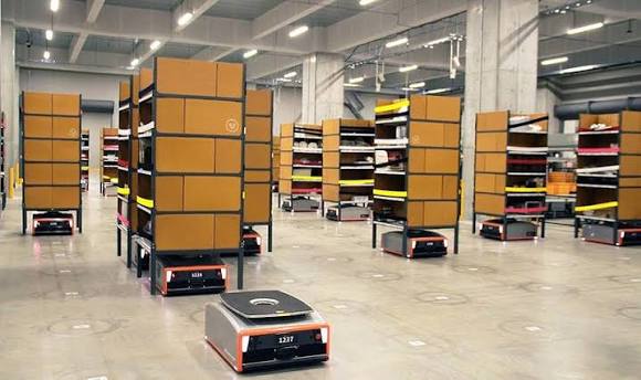
- ›Find packages, deliver to destination
- ›Sensors can't see through shelves
- ›Plan: where to look? When to act?
Simplified Version — Still Hard!
- ✗Walls block vision → partial observability
- ✗Package in any zone → uncertain state
- ✗Explore for info vs. act on belief
Sequential decisions under partial observability = POMDP
Solution: Online Planning with MCTS
Build a search tree at each timestep to select the best action
How It Works
- ›Build search tree from current belief
- ›Random rollouts estimate leaf values
- ›UCB guides which branches to explore
The Bottleneck
- ✗Noisy rollouts → poor value estimates
- ✗Blind exploration wastes search budget
- ✗Need many iterations to converge
Enhancing MCTS: Learned Guidance — and Its Catch
BetaZero: learn Vθ and Pθ to guide the search, AlphaZero-style — it works, but it doesn't scale
BetaZero Prior Work
- Vθ replaces noisy rollouts
- Pθ focuses search on promising actions
- Beats classical planners on long horizons
- Fixed-size belief vector → network tied to one problem size
The Training Deadlock
- Learning needs solved episodes — from an expert planner, or the learner's own search (self-play)
- Either way, training at size N means repeatedly solving size N — cost explodes with scale
- Deployment problems are large — exactly where guidance is needed most
What we need: learn on small problems, deploy on large ones
→ a belief representation whose learned knowledge transfers across problem sizes
Our Key Insight: Represent Beliefs as Graphs
A belief has structure — objects, attributes, actions, and their uncertainty. A fixed vector flattens it; a graph keeps it.
Fixed-Size Vector prior learned guidance
✗ Even where training works: every new size ⇒ new network ⇒ retrain
✗ And at large sizes it doesn't: training means solving large problems ⇒ the deadlock
Belief Graph GammaZero
Nodes & edges carry belief probabilities; the graph just grows.
✓ One network for every size — nothing to retrain
✓ Trains on small problems only — the deadlock never appears
One fix for both problems: learn entirely on small problems, deploy at any size
Belief-to-Graph Construction
GammaZero: Full Pipeline
Data Collection and Training
Deployment-size problems are never solved during training
Experimental Domains
4 POMDP benchmarks — partial observability, zero-shot generalization
LightDark(d)
1D localization. Visit light region to reduce uncertainty before reaching goal.
Test: LD(10)
RockSample(n,k)
n×n grid, k rocks of unknown quality. Noisy distance-dependent sensor.
Test: RS(15,15)–(25,25)
MultiObjectSearch
Find k hidden objects on n×n grid. Range-limited sensor.
Test: MOS(6,4)–(8,6)
Rearrangement
Locate k objects, transport to goals. Perception + manipulation.
Test: RG(6,4)–(8,5)
Results: Same-Size Performance
All methods trained and tested on identical sizes — Returns ± SE
Matches BetaZero
Comparable on shared domains (LD, RS) despite using a general graph architecture.
Results: Zero-Shot Generalization
Trained on small, tested on 2–6× larger — Returns ± SE. † = timeout
Zero-Shot Transfer
Train on small instances, deploy on 2–6× larger — no retraining needed.
What Patterns Does the GNN Learn?
The GNN learns relational patterns, not absolute positions.
Information Gathering
“High entropy on attribute nodes connected to a Check action → checking that rock has high information value.”
Same pattern applies whether 5 or 25 rocks.
Action Readiness
“Belief-weighted edges near the sample action indicate high-confidence state → sampling is worthwhile.”
Structural relationship, not domain-specific.
Why This Transfers
Patterns are about graph structure — connectivity, edge weights, node neighborhoods — not coordinates or object IDs.
Adding more objects extends the graph; same patterns apply.
What This Unlocks
Remember the deadlock: to guide search at scale, you first had to solve problems at scale
The Deadlock, Broken
Before: learned guidance existed only at sizes you could afford to solve, over and over, during training.
Now: train once on tractable instances → guide search on problems 2–6× larger than anything solved during training — no retraining.
Next Stop: Real-World Rearrangement
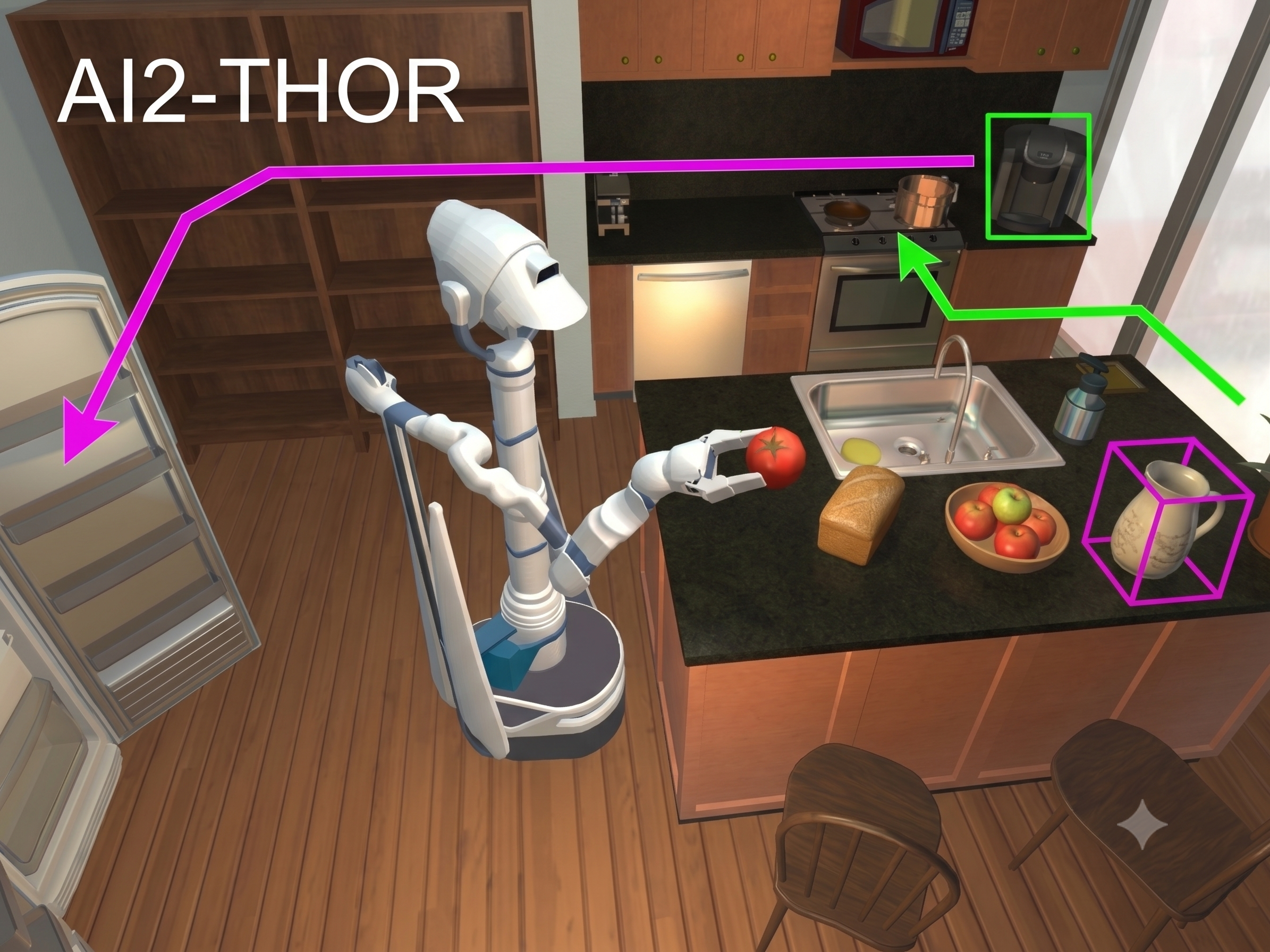
POMDP planning already tackles household object search & rearrangement (shown: AI2-THOR) — but planning speed is the bottleneck. Size-invariant learned guidance is a path to making it practical.
Benchmarks here are simplified — but the representation applies to any object-centric POMDP
Summary & Impact
Belief-to-graph construction — represents beliefs as uncertainty-aware graphs that scale with the problem
Matches or beats baselines on same-size tests — zero-shot generalization to 2–6× larger instances
Core Message
Represent the world — and its uncertainty — in a size-invariant way: learn from problems you can solve, generalize to the ones you can't.
Future: Real-world rearrangement — POMDP planning works there, but slowly. Learned guidance can make it practical.
Thank you! Questions?
Appendix
G + number to jump · T for slide navigator
Node Types: V = Vobj ∪ Vattr ∪ Vact ∪ {vglobal}
- Object nodes Vobj — all distinct entities; unifies movable entities (robot, box, package) and spatial entities (rooms, hallways, waypoints). Persist across all beliefs; serve as the valid arguments for actions and attributes; encode type (e.g. is_location, is_item) and static attributes.
- Attribute instance nodes Vattr — one node per attribute–value assignment that holds with sufficient probability, e.g. At(robot) = kitchen. Created selectively only when particle support ≥ τ.
- Action nodes Vact — parameterized actions, e.g. move(?from, ?to), pick(?object); applicability read off their connections to entities and condition nodes.
- Global node vglobal — maintains a holistic representation of the belief and propagates information across distant nodes in the graph.
Why this structure: separates persistent elements (entities, actions) from belief-dependent ones (attribute instances); unifying locations and objects treats navigation and manipulation as similar operations; selective attribute creation handles multimodal beliefs — if the robot is plausibly in the kitchen or hallway, both At-nodes exist, with edge weights carrying their probabilities.
Belief-Driven Sparsity: the Threshold τ
Attribute nodes are instantiated only with sufficient particle support — not all possible groundings
- Topology encodes the belief — a node's existence itself implies plausibility.
- Reduces computation — no nodes for unlikely hypotheses.
- Learn from structure — patterns come from structural presence/absence, not only numerical features.
RockSample example (τ = 0.3): At(robot,(1,1)) = 1.0 → node; IsGood(R1) = 0.40 and IsGood(R2) = 0.75 → nodes; their complements IsBad(R1) = 0.60, IsBad(R2) = 0.25 — the 0.25 falls below τ and is not instantiated.
Edge Types: E = Eattr-obj ∪ Eact-obj ∪ Eattr-act
- Attribute ↔ Object — each attribute node connects to the object it describes (owner) and to the node representing its value: At(robot) = kitchen links to both robot and kitchen. Edge features distinguish the two roles; edge weights carry the belief probability of the assignment.
- Action ↔ Object — actions link to objects that can serve as their parameters, capturing applicability constraints and expected outcomes. E.g. an edge from check(?rock) to rock3 encodes that rock3 can be checked, plus observation accuracy (decreasing with distance) and expected information gain.
- Attribute ↔ Action — attribute instances link to actions that require them as preconditions or produce them as effects, encoding how current beliefs constrain future actions and their outcomes.
Three functions: belief-weighted relationships (edge weight = strength of belief) · action-specific context (e.g. co-location requirements for sampling) · particle-support metadata separating confident beliefs from uncertain hypotheses.
Edge Features
- φtype ∈ {0,1}10 — one-hot edge type; bidirectional edges get distinct types to capture directionality.
- φrole ∈ {0,1}2 — for attribute edges: connects to the owner object vs. the value node.
- φbelief ∈ [0,1] — continuous probability: Σi wi · 1[relationship holds in si].
- φsupport — categorical consensus level: unanimous (>95%) · strong (70–95%) · weak (30–70%) · split (<30%).
Why both φbelief and φsupport? They derive from the same particle support, but the categorical version is an inductive bias: explicit signal for patterns like “split support ⇒ information-gathering is valuable.” E.g. IsGood(rock1) at φbelief = 0.72 is strong, while 0.68 is weak — the transition is salient even though the values are close. A sufficiently expressive GNN could learn such boundaries from φbelief alone; the categorical feature makes them easier to learn from limited data.
GNN: L Rounds of Message Passing
vi(l+1) = φv([vi(l), AGG({eij(l+1) : j ∈ N(i)}), g(l)])
g(l+1) = φg([g(l), AGG({vi(l+1)}), AGG({eij(l+1)})])
- φe, φv, φg are learned update functions; AGG is attention-weighted aggregation.
- The global node g enables rapid information propagation across distant nodes — crucial for maintaining performance as problem size increases.
Shared encoder, separate MLP heads (rather than independent networks): avoids redundant feature learning and halves inference cost during MCTS.
Expert Data Generation & Loss
Supervised learning: Vθ : B → ℝ and πφ : B × A → [0,1] from tuples (bi, vi*, πi*)
- Run optimal or near-optimal planners on small instances where exact solutions are computationally feasible.
- At each belief: query expert for action and Q-values → execute in environment → update belief from the received observation.
- After the episode: compute discounted returns by backward induction, associating each visited belief with its value-to-go (Algorithm 3).
Mean squared error for value prediction + cross-entropy for action classification, with weighting coefficients λv, λp. Leverages existing planning algorithms to generate high-quality training targets.
MCTS Integration: Three Enhancements
- Action prioritization — node expansion samples from the learned policy instead of uniformly: a ∼ Pθ(·|φ(b))
- Value estimation — leaf nodes evaluated by network lookup instead of expensive rollouts: v = Vθ(φ(b))
- Root action selection — combines visit counts with Q-values: π(a|b) ∝ N(b,a)zn · exp(Q(b,a))zq
Tree traversal uses PUCT adapted from AlphaZero to the belief-space setting:
Per simulation: sample s ∼ b → step to get (s′, o, r) → weighted particle belief update b′ → add node if b′ ∉ T → convert G′ = φ(b′) → recurse → backpropagate N(b,a) and running Q(b,a).
Implementation Details
Architecture & Search
- GNN encoder with shared MLP heads
- PUCT with progressive widening
- Per-domain constants → slides 38–40
Training
- 2–4 hours per domain on an RTX 3080
- 5 runs per configuration; best-performing setting reported
Evaluation
- Average discounted return over 100 episodes, different random seeds
- Reported as mean ± standard error
Generalization training protocol: LightDark — train on size 5, test on 10. RockSample — train on 5×5 to 10×10 grids with 5–10 rocks; test on (15,15), (20,20), (25,25). MOS & Rearrangement — train on grid sizes 3–4 with 2–3 objects; generalize to grid sizes 5–8 with 3–6 objects.
Ablation: Policy & Value Networks Alone
| Domain | Full (MCTS) | Raw Pθ | Raw Vθ* |
|---|---|---|---|
| LightDark(10) | 17.5 ± 1.2 | 14.4 ± 1.3 | 13.3 ± 1.4 |
| RockSample(15,15) | 20.5 ± 0.8 | 11.1 ± 2.0 | 9.1 ± 2.2 |
| MOS(5,3) | 18.0 ± 1.5 | 10.8 ± 1.8 | 9.9 ± 2.0 |
| Rearrange(5,2) | 12.5 ± 2.0 | 5.6 ± 2.2 | 6.3 ± 2.0 |
* one-step look-ahead using only the value network. Same-size setting (Table 1).
Findings: the policy network alone (no MCTS) reaches 60–80% of full performance; one-step look-ahead with the value network performs slightly worse. The combination through MCTS is consistently best — the two networks provide complementary guidance.
Full Results: Same-Size (Table 1)
All methods trained and tested on the same problem size — Returns ± SE
| Domain | GZ Full | GZ Raw Pθ | GZ Raw Vθ* | BZ Full | BZ Raw Pθ | BZ Raw Vθ* | POMCPOW | DESPOT | AdaOPS |
|---|---|---|---|---|---|---|---|---|---|
| LD(10) | 17.5±1.2 | 14.4±1.3 | 13.3±1.4 | 16.17±1.58 | 13.98±1.08 | 12.45±1.13 | 1.08±0.53 | 0.73±0.44 | 6.28±2.03 |
| RS(15,15) | 20.5±0.8 | 11.1±2.0 | 9.1±2.2 | 19.87±0.91 | 11.04±0.88 | 9.44±0.55 | 11.01±0.67 | 18.83±0.81 | 20.53±0.81 |
| MOS(5,3) | 18.0±1.5 | 10.8±1.8 | 9.9±2.0 | — | — | — | 7.5±1.5 | 6.4±1.8 | 15.5±2.0 |
| RG(5,2) | 12.5±2.0 | 5.6±2.2 | 6.3±2.0 | — | — | — | 4.3±1.5 | 3.4±1.5 | 7.7±2.0 |
* one-step look-ahead using only the value network. “—” = unsupported domain: BetaZero only supports LightDark and RockSample.
Full Results: Zero-Shot Generalization (Table 2)
GammaZero trained on small problems only; classical baselines run per-size — Returns ± SE
| Test Domain | GZ Full | GZ Raw Pθ | GZ Raw Vθ* | POMCPOW | DESPOT | AdaOPS |
|---|---|---|---|---|---|---|
| LightDark(10) | 15.2±1.5 | 12.1±1.6 | 11.2±1.7 | 1.08±0.53 | 0.73±0.44 | 6.28±2.03 |
| RockSample(15,15) | 17.8±1.2 | 11.1±2.0 | 9.1±2.2 | 11.01±0.67 | 18.83±0.81 | 20.53±0.81 |
| RockSample(20,20) | 10.2±1.8 | 5.4±1.0 | 4.4±2.0 | 9.92±0.67 | 0.0±0.0† | 10.96±0.78 |
| RockSample(25,25) | 3.5±2.0 | 4.8±1.2 | 3.9±1.5 | 2.1±0.8 | 0.0±0.0† | 4.2±1.0 |
| MOS(6,4) | 14.5±1.8 | 8.8±2.0 | 8.1±2.2 | 5.5±1.6 | 4.8±1.8 | 12.2±2.0 |
| MOS(7,5) | 11.2±2.0 | 6.5±2.2 | 6.0±2.3 | 3.8±1.8 | 3.2±2.0 | 9.0±2.2 |
| MOS(8,6) | 8.0±2.2 | 4.8±2.5 | 4.5±2.5 | 0.0±0.0† | 0.0±0.0† | 5.8±2.5 |
| Rearrange(6,4) | 9.2±2.0 | 4.5±2.3 | 5.0±2.2 | 3.0±1.6 | 2.4±1.8 | 5.8±2.0 |
| Rearrange(7,4) | 6.8±2.2 | 3.2±2.5 | 3.8±2.3 | 0.0±0.0† | 0.0±0.0† | 4.0±2.2 |
| Rearrange(8,5) | 4.5±1.8 | 2.2±1.6 | 2.8±1.5 | 0.0±0.0† | 0.0±0.0† | 2.9±1.7 |
* one-step look-ahead. † search timeout/failure. BetaZero cannot run zero-shot at all (fixed input dimensions).
Graceful Degradation with Scale
- RockSample scaling: 17.8 → 10.2 → 3.5 across (15,15) → (20,20) → (25,25) — despite never training beyond 10×10.
- At (25,25), all methods struggle with timeouts — and the raw policy network alone is the best performer (4.8 ± 1.2): structural patterns learned on small instances transfer even when search itself becomes intractable.
- Performance degrades gradually, not catastrophically, as size exceeds the training distribution — fixed-dimensional approaches cannot process out-of-distribution inputs at all.
Why: graph construction principles are identical at every size. Adding rocks simply adds object nodes and attribute instances — graph topology and edge types are unchanged, so the same GNN weights process problems of arbitrary scale.
Domain Details & State-Space Sizes
- LightDark(d) — 1D localization under state uncertainty; noisy observations improve near a “light” region at distance d. Larger d requires longer-horizon information gathering.
- RockSample(n,k) — n×n grid, k rocks of unknown quality; distance-dependent noisy sensor. |S| = O(n² · 2k) — from 12,800 states at (7,8) to over 400 million at (20,20).
- MultiObjectSearch(n,k) — find and declare k hidden objects with a range-limited sensor with detection probability ε. |S| = O(n2(k+1) · 2k).
- Rearrangement(n,k) — mobile manipulation domain introduced for this evaluation: locate k objects with unknown positions and transport them to goal locations. |S| = O(n2(k+1) · 4 · 2k) — perceptual uncertainty combined with multi-step planning.
Baselines
- BetaZero (Moss et al. 2024) — state-of-the-art learning-based POMDP planner: offline policy/value networks from expert demonstrations + online MCTS. Requires separate training for each problem size due to its fixed-dimensional belief representation.
- POMCPOW (Sunberg & Kochenderfer 2018) — extends POMCP to continuous observation spaces via progressive widening; tested with domain-specific heuristics.
- DESPOT (Ye et al. 2017) — scenario sampling builds a sparse belief tree; regularization balances policy size against estimated value.
- AdaOPS (Wu et al. 2021) — adaptively adjusts particle beliefs to maintain value function bounds; tested with fixed bounds on problems where QMDP is intractable.
Limitation: Object-Centric Scope
- Scope is object-centric POMDPs: the state must decompose into discrete entities with typed attributes and inter-entity relations (e.g. spatial adjacency, prerequisite dependencies).
- Graph construction assumes Vobj is known at planning time.
- Domains where objects appear, disappear, or have unknown cardinality would require dynamic graph construction.
Within scope, the schema (object types, attribute types, action types) is defined once per domain — graphs are then constructed automatically from any belief state.
Limitation: Independent Per-Attribute Marginals
- The graph approximates the joint belief through independent per-attribute distributions — particle weights are aggregated per attribute-value pair.
- Inter-attribute correlations are not preserved: two beliefs with identical marginals but different correlations produce the same graph.
- Paper's example: a correlation like “all objects are co-located” present in the particles is lost in the graph.
- Capturing joint structure would require higher-order representations such as hyperedges.
Illustration of the paper's example: belief A — 50%: all objects in room X, 50%: all in room Y (perfectly correlated). Belief B — each object independently 50/50 between X and Y. Identical marginals ⇒ identical graphs, though the joint beliefs differ.
Limitation: Discrete Action Spaces
- The current formulation assumes discrete action spaces — each grounded action is a node in Vact.
- Extending to continuous actions requires modifications to the action-node representation.
- Listed as a future direction alongside continuous state spaces.
Relation to Prior Work
- Learning for online POMDP planning (BetaZero, ConstrainedZero, LeTS-Drive) — learn offline, guide online search; all rely on fixed-size belief representations predetermined per domain. GammaZero's graphs handle variable-sized problems and capture action–state relationships.
- Classical online planners (POMCP, POMCPOW, DESPOT, AdaOPS) — rely on domain-specific heuristics for value estimation and action selection; GammaZero learns these instead.
- Generalized classical planning — GPL: globally consistent value estimates get harder at scale; ASNets: fixed-depth architecture limits long dependency chains; GRAPL: no explicit action-object / parameter-dependency modeling.
- GABAR (Mangannavar et al. 2025) — action-centric graphs with GNN encoder + GRU decoder for deterministic planning; strong generalization but cannot handle belief uncertainty. GammaZero extends the graph representation to POMDPs: encode belief uncertainty while preserving the structural patterns that enable generalization.
Future Directions
- Hierarchical graph representations for extreme-scale problems.
- Continuous state and action spaces.
- Self-supervised learning to reduce dependence on expert demonstrations.
From the paper's conclusion. Dynamic graph construction (for open-world object sets) and hyperedges (for joint belief structure) also appear as needed extensions in the Limitations discussion.
Search Budget: 1000–2000× Fewer Simulations
| Method | Simulations at Evaluation | Notes |
|---|---|---|
| GammaZero (ours) | 50–100 | 100 for RockSample, 50 default for LightDark |
| BetaZero | 100 | same PUCT solver |
| POMCPOW (LightDark) | 100,000 | + 1 s wall-clock limit |
| POMCPOW (RockSample) | 200,000 | + 1 s wall-clock limit |
| AdaOPS | wall-clock budgeted | 1 s time limit |
| DESPOT | wall-clock budgeted | 1 s time limit |
Values from the experiment configurations.
Takeaway: comparable or better results with 1000–2000× fewer simulations than POMCPOW — the learned GNN makes each simulation count far more.
Same Base Search — Only the Representation Differs
- GammaZero and BetaZero use the exact same base MCTS algorithm (PUCT): same solver code, same particle-filter infrastructure.
- If the base algorithm explained the results, the two would be identical — Table 1 shows GammaZero matches or beats BetaZero at the same size. The difference is the graph representation.
- BetaZero's search is actually tuned harder on RockSample: c = 50, depth = 15, progressive widening disabled — GammaZero evaluates with c = 1.0, depth = 10.
- Ablation: the raw policy network with no MCTS at all reaches 60–80% of full performance — if search were doing the heavy lifting, that column would be near zero.
Sound bite: “GammaZero and BetaZero share the exact same PUCT implementation. The only difference is the belief representation — fixed-size MLP vs. our graph.”
Baselines Use Hand-Crafted Heuristics — We Use None
- POMCPOW — LightDark: Local Approximate Value Iteration heuristic (1,000 iterations, 1,000 samples); RockSample: RSExitSolver (“move east”) heuristic.
- AdaOPS — lower bound: random-rollout value / RSExitSolver; upper bound: LAVI approximation / QMDP (fully observable relaxation).
- DESPOT — lower bound: random rollout / RSExitSolver rollout; upper bound: problem-specific / fully observable value bound (QMDP); default action: RSExitSolver.
- GammaZero — replaces all of these with the learned GNN: no hand-crafted value bounds, no domain rollout policies.
Sound bite: “The baselines use QMDP upper bounds and exit-strategy heuristics hand-crafted for each domain. We use zero domain heuristics — only the learned GNN.”
GammaZero: MCTS Parameters per Domain
| Parameter | LightDark | RockSample | MOS | Rearrangement |
|---|---|---|---|---|
| Sims — training data collection | 10 | 500 | 500 | 15,000 |
| Sims — evaluation | 50 (default) | 100 | 20,000 | 25,000 |
| Particles | 1,000 (default) | 1,000 | 1,000 | 1,500 |
| Exploration c (train) | 4.0 | 4.0 | 100.0 | 1,500.0 |
| Exploration c (eval) | 1.0 | 1.0 | 1,000.0 | 1,500.0 |
| k_action | 2.0 | 2.0 | 20.0 | 30.0 |
| α_action | 0.25 | 0.25 | 0.25 | 0.25 |
| k_state | 2.0 | 2.0 | 20.0 | 30.0 |
| α_state | 0.1 | 0.1 | 0.1 | 0.1 |
| Tree depth | 10 | 10 | 10 | 10 |
| Discount γ | 0.99 | 0.99 | 0.95 | 0.95 |
From the experiment configurations.
GammaZero: GNN Architecture per Domain
| Parameter | LightDark | RockSample | MOS | Rearrangement |
|---|---|---|---|---|
| Hidden dim | 128 | 256 | 512 | 512 |
| Message-passing rounds L | 5 | 5 | 6 | 7 |
| Attention heads | 8 | 8 | 8 | 8 |
| MLP layers (per head) | 2 | 2 | 3 | 3 |
| Dropout | 0.1 | 0.1 | 0.1 | 0.1 |
| Attention dropout | 0.2 | 0.2 | 0.2 | 0.2 |
| Node feature dim | 16 (default) | 100 | 150 | 180 |
| Edge feature dim | 4 (default) | 40 | 60 | 80 |
| Global feature dim | 16 (default) | 100 | 150 | 180 |
From the experiment configurations.
GammaZero: Training Hyperparameters
| Parameter | LightDark | RockSample | MOS | Rearrangement |
|---|---|---|---|---|
| Epochs | 100 | 100 | 150 | 200 |
| Batch size | 32 | 32 | 32 | 32 |
| Learning rate | 1e-4 | 1e-4 | 1e-4 | 5e-5 |
| Weight decay | 1e-4 | 1e-4 | 1e-4 | 1e-4 |
| Optimizer | Adam | Adam | Adam | Adam |
| Replay buffer size | 50,000 | 50,000 | 100,000 | 150,000 |
| Value / policy loss weights | 0.5 / 0.5 | 0.5 / 0.5 | 0.5 / 0.5 | 0.5 / 0.5 |
| Train / validation split | 80 / 20 | 80 / 20 | 80 / 20 | 80 / 20 |
Value loss: MSE · policy loss: cross-entropy · dynamic loss scaling: EMA α = 0.9 · hardware: RTX 3080, 2–4 h per domain.
BetaZero Configuration (Direct Competitor)
| Parameter | LightDark | RockSample |
|---|---|---|
| MCTS solver | PUCT (same codebase) | PUCT (same codebase) |
| MCTS simulations | 100 (default) | 100 |
| Exploration c | default (1.0) | 50.0 |
| Progressive widening | default (enabled) | disabled entirely |
| Tree depth | 10 (default) | 15 |
| Particles | 500 | 1,000 |
| Network | MLP (fixed-dim input), layer 64 | MLP (fixed-dim input), layer 128 |
| Epochs / batch / LR | 50 / 1,024 / 1e-4 | 10 / 1,024 / 1e-3 |
| Optimizer / dropout | Adam / 0.2 | RMSProp / 0.5 (+ batchnorm, m=0.7) |
| L2 / Dirichlet noise | 1e-5 / α=0.03, ε=0.25 | 1e-5 / α=0.03, ε=0.25 |
Cannot generalize to new problem sizes — requires retraining per size. Note the harder-tuned search on RockSample (c=50, depth=15, no widening).
Classical Baseline Configurations
POMCPOW
- Tree queries: 100k (LD) / 200k (RS), max 1.0 s
- Criterion: MaxUCB(10.0); depth 20 (LD) / default (RS)
- k_obs 4.0 / 1.0; α_obs 0.03 / 1.0; action widening enabled (LD) / disabled (RS)
- Heuristics: LAVI (LD); RSExitSolver “move east” (RS)
AdaOPS
- m_min: 10 (LD) / 100 (RS)
- δ: 1.0 (LD) / 0.1 (RS)
- Lower bound: random rollout (LD) / RSExitSolver (RS)
- Upper bound: LAVI (LD) / QMDP (RS)
DESPOT (AR)
- λ: 0.1 (LD) / 0.0 (RS); K scenarios: 30 / 100
- Lower bound: random rollout / RSExitSolver rollout
- Upper bound: problem-specific / fully observable (QMDP)
- Default action: random / RSExitSolver
From the experiment configurations. All classical baselines run per-size with these domain-specific bounds and heuristics.